
Hybrid retrieval: dense, sparse and graph over internal documents
14 min read15 sections
Hybrid retrieval is not adding dense and BM25 scores together. This post walks through each decision: BGE-M3's three representations, RRF, DBSF, retrieve-then-rescore, chunking, graphs and query rewriting — with the cost of each choice.
In this post
- Why dense vectors alone are not enough for internal documents
- Where keywords win: queries full of identifiers
- One encoder, three representations (BGE-M3)
- The evidence: learned sparse mode versus BM25 (figure)
- Why you cannot add dense and BM25 scores directly
- RRF: merging by rank, not by scale
- Weighted RRF and DBSF: two options when rank is not enough
- Choosing and tuning weights without fooling yourself
- The cost of fusion: a tax on every query
- Multi-stage retrieval: retrieve coarse, then rescore
- Chunking decides evidence quality
- Graphs: when a third branch is worth it
- Rewriting follow-up questions
- Where OpenVie implements these
- In short
Why dense vectors alone are not enough for internal documents
Dense retrieval encodes the query and the passage as two nearby points in an embedding space. It is strong at paraphrase: ask how to change your password and it still finds the passage about resetting it. But internal documents are not only natural prose.
Internal documents carry error codes, contract numbers, abbreviations, version tags, product codes and people's names. On those identifiers, embeddings often fail quietly: OVK-2291 and OVK-2219 look almost identical as vectors but mean entirely different things, and a string like ERR_403_TENANT may carry no meaning for the model to grasp.
- Queries with rare identifiers: the embedding model never saw that token in training, so the vector is close to meaningless.
- Queries matching a rare but exact term: a document ID, an error code, a clause number.
- Short queries with little context: dense needs context to infer intent, but the user typed three words.
You do not need to drop dense. You need a second branch that counts words. That is the entire reason hybrid retrieval exists: two different views of the same corpus, not one better method replacing the other.
Where keywords win: queries full of identifiers
Keyword retrieval, typically BM25, scores on term frequency and how rare a term is across the corpus. It does not understand semantics, but it matches exactly. On an all-identifier query, that is precisely what you want.
Picture a query like: which version did this error show up in, under which ticket, in which workspace. It contains a product name, a version number and a ticket ID. Dense may return passages that talk generally about timeout errors, sounding plausible but citing the wrong document. BM25 only has to see the exact code to lift the right passage to the top.
- Queries with error codes, ticket IDs, contract numbers or version numbers: keywords win clearly.
- Queries rephrased with synonyms and no rare terms: dense wins.
- Queries mixing both: you need both branches, and you need a sane way to merge them.
The key point is that internal documents rarely belong to just one category. A real operations corpus always holds both prose and identifiers, often in the same document. So the question is not dense or sparse, but how to combine them without wrecking the ranking of either.
One encoder, three representations (BGE-M3)
BGE-M3 is a multilingual encoder that produces three representations for the same input. From a single pass you get three different views of a passage, instead of operating three separate models.
- A dense vector: one point for the whole passage, used for approximate semantic search over a vector index.
- Learned sparse weights: a weight per token, enabling exact keyword-style matching that the model learns instead of counting by hand.
- Multi-vector ColBERT-style embeddings: one vector per token, used when you need finer rescoring.
Because dense and sparse come from the same encoder, they share a tokenizer and a representation space. That makes operations simpler: one model, one inference pass, two indexes built from the same source. You still store two indexes — one for vectors, one for sparse weights — but you are not synchronising two unrelated pipelines.
The evidence: learned sparse mode versus BM25 (figure)
The natural question is whether the learned sparse branch is genuinely worth adding or is just BM25 in new clothes. The BGE-M3 report publishes a direct comparison between BM25 and M3's sparse mode across three multilingual datasets.
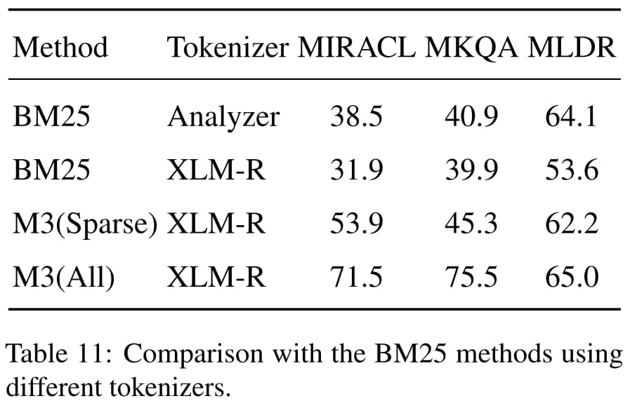
Table 11 from the BGE-M3 report. On MIRACL and MKQA, M3(Sparse) beats BM25 with the Analyzer tokenizer (53.9 and 45.3 versus 38.5 and 40.9); on MLDR, BM25 still edges ahead (64.1 versus 62.2). M3(All) — using all three representations — wins every column (71.5 / 75.5 / 65.0).
Read down each column to see the pattern. On MIRACL, M3(Sparse) reaches 53.9 against 38.5 for BM25 Analyzer and 31.9 for BM25 XLM-R — a wide gap. On MKQA, M3(Sparse) reaches 45.3, ahead of both BM25 variants. Only on MLDR does BM25 Analyzer edge up to 64.1 against 62.2 for M3(Sparse).
The lesson is not that learned sparse always wins. The lesson is that replacing BM25 with a learned sparse branch has support, and that combining all three representations (M3(All)) tops every column. In other words, hybrid is not a fallback — it is the best configuration in this table.
Why you cannot add dense and BM25 scores directly
The first reflex with two branches is to add their scores with an alpha weight. It is popular because it is simple, but it rests on a false assumption: that the two score scales can be compared directly.
A cosine score is bounded to a fixed range. A BM25 score is not bounded: it depends on document length, term frequency and rarity, so it can jump from a few units to dozens between two different queries. Add them with a fixed weight and whichever branch has the larger amplitude dominates the other — and which branch dominates changes from one query to the next.
Cosine is bounded to a range; BM25 is not. Adding two different score scales with a linear alpha is not trustworthy, especially when the scale itself shifts from query to query.
The Qdrant documentation says this outright: a linear alpha combination of dense and BM25 scores is not reliable. The problem is not that you picked the wrong alpha; it is that one fixed coefficient cannot normalise two score distributions that keep moving. This is exactly why rank-based fusion methods exist.
RRF: merging by rank, not by scale
Reciprocal Rank Fusion (RRF) ignores the score values and uses only ranks. Each branch returns a ranked list; RRF sums the reciprocal rank of each document across branches to produce a final score.
score(d) = Σ_branches 1 / (k + rank_branch(d)) // Qdrant: k defaults to 2, and is configurable// only ranks are needed, not raw scoresBecause it uses only ranks, RRF is immune to score-scale differences. A document ranked first on the dense branch and third on the sparse branch gets lifted, while a document appearing on only one branch still scores but lower. The constant k softens the influence of the top ranks: a small k lets top-1 dominate more, a large k flattens the contribution across ranks.
RRF's weakness is that it throws away confidence information. Two documents far apart in score can be one rank apart, so RRF treats them almost the same. That is the price of stability, and the reason the variants below exist.
Weighted RRF and DBSF: two options when rank is not enough
When you have reason to trust one branch more than the other, weighted RRF lets you assign a coefficient to each branch before summing. The final score is a weighted sum of the reciprocal-rank contributions. It is still rank-based fusion; it just uses weights to express confidence.
DBSF (Distribution-Based Score Fusion) goes the other way: it uses raw scores but normalises each branch's score distribution by three standard deviations around the mean, then sums the normalised scores. If every score in a branch is equal, DBSF returns 0.5 for that branch, avoiding a divide by zero variance.
- You have an eval set to tune on: use weighted RRF.
- You trust the relative magnitude of raw scores: use DBSF.
- You have nothing to measure and want a safe default: use RRF.
These three selection rules come from the Qdrant documentation and match intuition: rank-based fusion is the default because it assumes nothing about scale; DBSF is only for when you genuinely trust raw scores; and weighted RRF is only worth using when you have evidence to set the weights.
Choosing and tuning weights without fooling yourself
The weights in weighted RRF are a parameter, and any parameter can be over-tuned. If you measure quality on the very set you used to tune the weights, the result looks better than reality. That is not an improvement; it is self-deception.
- Split the evaluation set into two separate halves.
- Tune the weights on one half.
- Measure on the other half, which was never used for tuning.
- Accept the configuration only if it wins on the held-out half.
Weights are also not a permanent constant. The Qdrant documentation recommends re-tuning after you change the retriever, change chunking, or when the corpus drifts — new documents shift the score distributions. A weight that was good this month can drift off next month.
The practical path is to start from unweighted RRF, measure, and only add weights once the data shows one branch is genuinely stronger on your query mix. Do not start by tuning three parameters at once on a small set.
The cost of fusion: a tax on every query
Fusion is not free. An analysis called The Fusion Tax, measured over seven BEIR datasets and three fusion functions, shows that even the best method — dense-weighted score interpolation — still ranks a relevant document below its better branch on 13–48% of queries, and below dense-only on 8–21%.
A few observations come with it. RRF pays a higher tax when one branch is much stronger than the other, because averaging drags the strong branch down. The loss is mostly a ranking effect rather than lost recall: the relevant document stays in the result set, it just sinks. It shows up most on queries that only one branch can cover.
There is a partial mitigation: cross-encoder rescoring. But a cross-encoder only recovers part of the loss, and only where it is itself reliable. If the correct document was pushed out of the candidate set, the cross-encoder has nothing to score.
Multi-stage retrieval: retrieve coarse, then rescore
One way to control cost and quality is to split retrieval into two stages: a cheap first stage that gathers candidates, and a more expensive but more accurate second stage that rescores them. Qdrant supports this with nested prefetch: a sub-query runs first and its results feed the main query.
// stage 1: gather candidates with reduced vectors (byte/MRL)// stage 2: rescore with full vectors// or multi-vector ColBERT // vectors used only for rescoring can disable HNSW:// m = 0The idea is that reduced vectors (byte quantization, or MR L dimension truncation) are good enough for fast coarse filtering, but not precise enough for the final ordering. You pull a wide candidate set with reduced vectors, then rescore that small set with full vectors or with multi-vector ColBERT, which scores token by token and is more accurate but more expensive.
One operational detail: vectors used only for rescoring do not need an approximate-nearest-neighbour graph index. Disabling HNSW with m=0 for those vectors saves memory, because they never take part in coarse search. It is a small optimisation, but worth doing when you rescore full vectors over the whole candidate set.
Chunking decides evidence quality
Every retrieval branch is only as good as the unit of text it returns. If the passage does not contain the answer, no ranking function can save you. Chunking is the decision that sits before both dense and sparse, and it sets the evidence quality for everything downstream.
- Overlap gave no measurable benefit and only raised index cost — on Natural Questions with SPLADE and Mistral-8B, the overlap did not improve quality enough to justify it.
- Sentence-based chunking is the most cost-effective option, on par with semantic chunking up to about 5k tokens.
- There is a context cliff: past roughly 2.5k tokens, quality drops.
- Optimal context depends on the goal: semantic quality peaks at small context, while exact match needs larger context.
This is convenient operationally: sentence-based chunking is a cheap, sensible starting point, instead of building a complex semantic splitter. But note the 2.5k cliff — it explains why padding each chunk with more context often backfires. And because different goals need different sizes, do not assume one chunking setup serves both semantic QA and exact-match lookup well.
Graphs: when a third branch is worth it
The knowledge graph is the third branch, and also the one most easily added wastefully. Evidence from GraphRAG-Bench shows the graph is not a universal upgrade.
On simple fact-lookup questions, basic RAG is equal to or better than GraphRAG. The graph advantage only becomes clear as questions grow more complex: multi-step reasoning, synthesising scattered context, and generating new content from information spread across documents.
- On a novel dataset (long text), that complex question group reached 87.9–90.9% evidence recall with one graph implementation.
- Token cost rises sharply: the community-summary variant pushes prompts into the tens of thousands of tokens or more.
- A leaner variant — without community summaries — keeps prompts around 10^3 tokens.
The right reading is: the graph is a conditional tool. If your users mostly ask fact lookups, adding a graph only costs money. If they ask multi-step questions spanning many documents, a graph may be worth it — as long as you accept the far higher token consumption and pick a lean enough variant.
Rewriting follow-up questions
In conversation, questions rarely stand alone. A user asks about one document, then the next turn says just what about the security part. Feed that raw sentence to the index and neither branch has anything to grip: it lacks a subject and an identifier.
Rewriting follow-up questions is the step that turns a shortened turn into a standalone query by pulling context from earlier turns. After rewriting, the sentence becomes a full query and both branches get a chance to return the right document. This is a standard component of a multi-turn hybrid pipeline, not just an interface trick.
- Keep the previous turns as context.
- Rewrite the current question into a self-contained query.
- Run the rewritten query through both the dense and sparse branches.
- Fuse the results and rescore.
Evidence from SemEval-2026 Task 8 backs this: a training-free hybrid pipeline combining dense and sparse with corpus cleaning, conversational query rewriting and reranking is a sensible configuration for multi-turn retrieval. None of those steps needs model retraining.
Where OpenVie implements these
OpenVie is a self-hosted, Vietnamese-first RAG platform released under Apache-2.0. The decisions above are not scattered across docs — they map to specific parts of the system.
- M4 — retrieval: hybrid dense + sparse + graph, with follow-up query rewriting and RRF rank fusion.
- M24 — embeddings: the default model runs locally via Ollama, with
bge-m3for embeddings; pointing at an external OpenAI-compatible endpoint is the operator's choice. - M8 — rescoring: the cross-encoder reranker (TEI) is optional and fails open on error, so its absence does not crash the retrieval flow.
- M9 — tenancy: Qdrant and Kuzu are always tenant-filtered, so the vector, graph and sparse branches all stay inside the same data boundary.
- M2 — citations: sources are shown only after an access check and the final response is persisted; drafts carry no source chips.
Two design choices stand out. First, M8 lets the reranker fail open: if the TEI service dies, retrieval still returns the fused results instead of erroring. Second, M24 makes local models the default, so the cost per query is one encoder pass plus rescoring passes, not an external API bill.
A note on scope: source code in the repo is not evidence of a production service, and deployment hardening must be verified in your own environment. The benchmark numbers in this post belong to the original sources, not to OpenVie's measurements on your corpus.
In short
Hybrid retrieval is a chain of decisions with clear costs, not an on/off switch. Every branch you add brings coverage and carries cost and ranking risk with it.
- Dense and sparse cover different query types; keywords win when the query holds identifiers.
- Do not add raw scores with a linear alpha — the scales are not comparable.
- RRF fuses by rank; weighted RRF and DBSF are the options when rank alone is not enough.
- Fusion has a tax: even the best method drops rank on 13–48% of queries across 7 BEIR datasets.
- Reranking, sentence chunking and query rewriting are cheaper levers than another branch.
- A graph is only worth it for complex questions; otherwise it just burns tokens.
If you remember one thing: measure on a held-out set, pick RRF as the safe default, and add complexity only when your data — not a benchmark — says it is worth it.
Sources
- The Fusion Tax: A Diagnostic Analysis of When Hybrid Retrieval Hurts — arXiv:2610.30612
- When to use Graphs in RAG (GraphRAG-Bench) — arXiv:2506.05690
- A Systematic Analysis of Chunking Strategies for Reliable Question Answering — arXiv:2601.14123
- Hybrid and Multi-Stage Queries — Qdrant documentation
- BAAI/bge-m3 — model card (HuggingFace)
- Training-free multi-turn hybrid RAG — SemEval-2026 Task 8